Trees, bagging, random forest, boosting and their implementations


A tree based model can be written as $f(x) = \sum_{m=1}^M c_m 1_{(x \in R_m)}$, where $c_m$ is the leaf node value of the region $R_m$.
Figure below show two cases, one where a linear model is better than a tree-based model (top row) and one where a tree-based model is better than a linear model (botton row).


- Step 1
- The goal is to find boxes $R_1, ... R_j$ that minimizes the $RSS=\sum_{j=1}^J \sum_{i \in R_j} (y_i - \hat{y}_{R_j})$, where $\hat{y}_{R_j}$ is the mean response for the training observations within $R_j$.
- It is computationally infeasible to consider every possible partition of the feature space into $J$ boxes.
- For this reason, we take a top-down, greedy approach that is known as recursive binary splitting.
- The approach is top-down because it begins at the top of the tree (at which point all observations belong to a single region) and then successively splits the predictor space.
- It is greedy because at each step of the tree-building process, the best split is made at that particular step, rather than looking ahead and picking a split that will lead to a better tree in some future step.
- In greater detail, for any $j$ and $s$, we define the pair of half-planes $R_1(j, s) = \{X|X_j < s\}$ and $R_2(j, s) = \{X|Xj ≥ s\}$, and we seek the value of $j$ and $s$ that minimize the equation $$\sum_{i: x_i \in R_1(j,s)}(y_i − \hat{y}_{R_1})^2 + \sum_{i: x_i \in R_2(j,s)}(y_i − \hat{y}_{R_2})^2$$
- Step 2
- Step 1 tends to overfit the training data.
- Computing the test error at each partition on step 1 is expensive. We use cost complexity pruning instead.
- For each value of $\alpha$ there corresponds a subtree $T \subset T_0$ such that $$ \sum_{m=1}^{|T|} \sum_{i: x_i \in R_m} (y_i − \hat{y}_{R_m})^2 + \alpha |T|$$ is as small as possible, where $|T|$ is the number of terminal nodes of the tree $T$ and $\alpha$ is a tunning parameter.
- It turns out that as we increase $\alpha$ from zero, branches get pruned from the tree in a nested and predictable fashion, so obtaining the whole sequence of subtrees as a function of $\alpha$ is easy.
- Uses recursive binary splitting to build the tree.
- Task can be to either return the most common class or to return the proportion of each class.
- There are a few possibilities to use instead of the RSS:
- classification error rate: $E = 1 - max_k(\hat{p}_{mk})$, where $\hat{p}_{mk}$ is the proportion that the $m$-th region are of class $k$.
- Gini index: $G = \sum_{k=1}^{K} \hat{p}_{mk} (1-\hat{p}_{mk})$
- Cross-entropy: $D = -\sum_{k=1}^{K} \hat{p}_{mk} \log \hat{p}_{mk}$
- When building a classification tree, either the Gini index or the crossentropy are typically used to evaluate the quality of a particular split, since these two approaches are more sensitive to node purity than is the classification error rate. Any of these three approaches might be used when pruning the tree, but the classification error rate is preferable if prediction accuracy of the final pruned tree is the goal.
- Advantages
- Tree-based methods are more interpretable
- Can handle qualitative predictors without the need to create dummy variables
- Disadvantages
- Decision trees by itself are in general not as accurate as other linear models
- Decision trees are not robust in the sense that an small change in the data can lead to a very different estimated tree. That is, decision trees have high variance.
Those are generic approaches that can be applied to many statistical learning methods.
Assume we have $n$ observations of training data, $Z$. Bootstrapping works by sampling with replacement B datasets with $n$ observations each $Z^{*1}$, ..., $Z^{*B}$. Those sampled datasets can then be used either to compate uncertainty measures or by averaging different model estimates to reduce the variance of the original model.
Ideally we would like to have B independent datasets, but when collecting independent datasets are not possible, bootstrapping can be used.
What are the bias introduced by bootstraping instead of using independent datasets?
- For regression, fit tree-based models on B bootstraped datasets and average the results.
$$\hat{f}_{\text{avg}}(x) = \frac{1}{B}\sum_{b=1}^{B} \hat{f}^b (x)$$
- For a classification tree we can predict the class of a data point by taking the majority vote between the B predictions.
- Each tree is grown deep, and are not pruned. Hence, each individual tree has high variance but low bias. The boostrap technique helps by reducing the variance.
- Out-of-bag test error estimation:
- On average, each bagged tree uses 2/3 of the original data.
- For each observation there are on average B/3 model that were not trained on it.
- If we average for regression and take the majority for classification of the predictions of those B/3 models, we have an out-of-bag (OOB) prediction for the i-th observation.
- If we do the above for all the observation we have the overall OOB MSE for regression or classification error for classification.
- The resulting OOB error is a valid estimate of the test error for the bagged model.
- It can be shown that with B sufficiently large, OOB error is virtually equivalent to leave-one-out CV error.
- Interpretability and variable importance
- We lose the easy of interpretation when bagging tree-based models
- We can compute feature importance by computing the average decrease in the error metric obtained by splits of the feature.
- Similar to bagging, except that when choosing which feature to split we randomly select $m$ out of the $p$ predictor to be considered.
- Usual choice $m = \sqrt p$
- $m = p$ means that random forest equal to bagging.
- The logic behind chosing a subset of the predictors before each split is to create more uncorrelated trees. Say there is a strong predictor that will be picked for all the trees when bagging, randomly selecting m predictor will give a change for other predictors to be considered, leading to more uncorrelated trees.
- Unlike bagging, boosting does not involve bootstrap sampling, instead the trees grows sequentially, where each tree is fit on a modified version of the original data set.
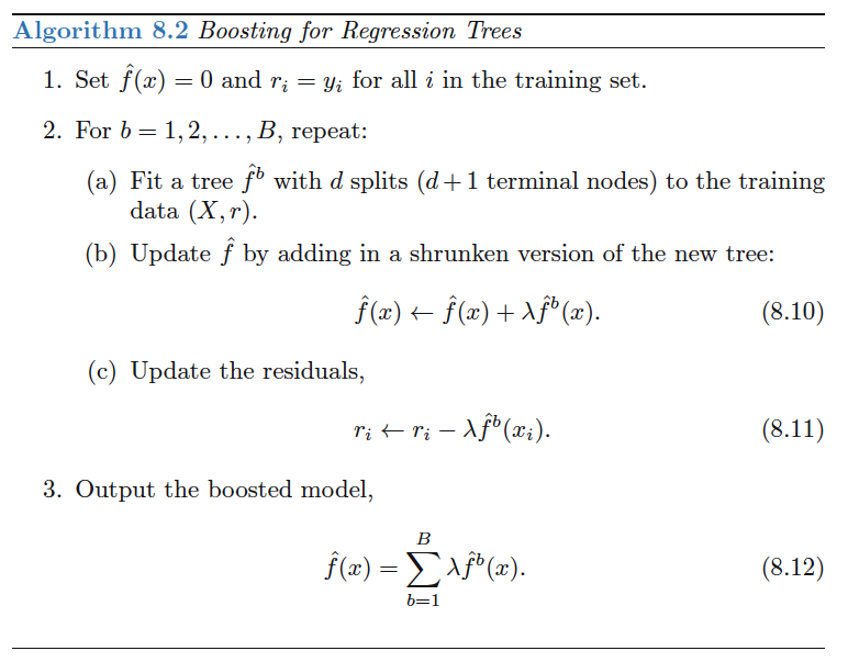
Boosting has three tuning parameters:
- The number of trees $B$. Unlike boosting and random forest we can overfit the data with high $B$, although it happens slowly if at all. We use CV to select $B$.
- The shrinkage parameter $\lambda$, a small positive number that controls the rate at which boosting learns. Typical values are $0.01$ or $0.001$ but the value is problem dependent. Smaller $\lambda$ can require larger $B$.
- The number $d$ of splits in each tree, which controls the complexity of the boosted ensemble. $d=1$ often works well and means that we are fitting an additive model since each tree involves only one predictor. More generally, $d$ is the interaction depth and controls the interaction order of the boosted model, since $d$ splits can involve at most $d$ variables.
-
Kaggle lightGBM notebooks
-
Home Credit Default Risk dataset
-
LightGBM with Simple Features
- Most of the script is feature pre-processing
- Uses LGBMClassifier with hyperparameter already tuned
- Uses sklearn CV
- Display feature importance
-
LightGBM with Simple Features
-
Home Credit Default Risk dataset
- LightGBM
- XGBoost
- LightGBM/XGBoost comparison
- XGBoost vs LightGBM: How Are They Different
- Set of LTR notebooks involving boosting from sophwatts
- Chapter 8 of Introduction to Statistical Learning
- Covered section 8.1 and 8.2
- Need to cover section 8.3